GIS 4048: Applications in GIS Module 7

Module 7:  Homeland Security – Protect

This week’s lab involved the summarizing of data in a table, performing the Generate Near Table analysis, Clipping the data frame, managing elevation data, working with LiDAR data, using the LAS Toolbar, the LAS Dataset to Raster Conversion Tool, the Hillshade Function, the Viewshed Analysis, using the 3D Analyst Extension, creating Lines of Sight, and working with ArcScene Viewer.

The maps below depict critical infrastructure, security checkpoints, surveillance locations, and lines of sight in the vicinity of the finish line for the Boston Marathon so that homeland security planners can implement protective measures such as securing the perimeter and stepping up surveillance posts at ingress and egress points. 

GIS 4102: GIS Programming Module 6

Module 6: Geoprocessing with Python

This week’s lecture covered using Python for geoprocessing tools, working with toolboxes, using functions and classes, using environment settings, working with tool messages and ArcGIS licenses, and accessing Help for syntax and sample code.

This week’s assignment involved writing a script to do the following:

1.     Add XY coordinates to a layer by using the AddXY Tool.

2.     Creating a buffer around features by using the Buffer Tool.

3.     Dissolving the buffer layer into a separate, single feature by using the Dissolve Tool.

4.     Printing the messages after each tool.

Below is a screen shot of the results in the Interactive Python window.

GIS 4048: Applications in GIS Module 6

Module 6:  Homeland Security – Prepare MEDS

One of the goals of the Department of Homeland Security (DHS) is to maintain a comprehensive geospatial database prepared, ready, available, and accessible to communities so they can prevent, prepare, respond and recover from a catastrophic event.  The Minimum Essential Data Sets (MEDS) is a geospatial dataset for homeland security planning and operations managed by the Homeland Security Infrastructure Program (HSIP).

MEDS data themes include:

Orthoimagery

Elevation -

Hydrology

Transportation

Boundaries

Structures

Geographic Names

Data should be two years current for urban areas and five years for large areas.  The data is used by various governmental agencies to prepare, prevent, respond and recover from a catastrophic event such as a terrorism attack.

This week’s lab assignment involved the compiling and manipulation of data to prepare a MEDS for the Boston Metropolitan Statistical Area (a tier 1 urban area) in anticipation of the Boston marathon.  Tier 1 urban areas are the largest, most populated metropolitan centers in the country. 

The starting datasets were downloaded from the USGS’s National Map Viewer and clipped to the Boston area of study.  A geodatabase was created and the data frame mapping environment was set including the creation of eight group layers to match the MEDS data themes above.  Datasets were manipulated, created and placed into the applicable group layer.

Some of the tools and procedures used in this lab include joining a table by attributes, setting labels to show only at specific scales, setting group layers, selecting by location to export data, working with various types of symbology and styles (like transportation specific style of symbology), setting layers to display at certain scales, extracting by mask from a raster, using colormaps, adding XY coordinate data as a layer, and saving to layer files to preserve symbology for future re-use.

GIS 4102: GIS Programming Module 5

Module 5: Geoprocessing in ArcGIS

This week’s assignment covered creating a toolbox, creating a tool using Model Builder, setting Model Parameters, exporting a script from Model Builder, updating that script to work outside of ArcMap and creating a script tool from it.

The tool does the following:

1.  Clips the Soils layer to the Basin features.

2.  Selects Not Prime Farmland from the Clip.

3.  Erases this selection from the original Basin layer.

4.  Creates a new Basin layer without the Not Prime Farmland clipped/selection.

Below is a screen shot of the output shapefile (the new Basin layer without the Not Prime Farmland).

GIS 4048: Applications in GIS Module 5

Module 5:  Homeland Security – DC Crime Mapping

This week’s lab involved the creation of two maps based on January, 2011 crime data for Washington, DC.  The lab covered the geocoding of addresses by creating a custom address locator, creation of graphs and reports, various types of symbology, the use of the multiple ring buffer tool, spatial joins, and the spatial analyst toolbox and kernel density.

The first map represents crime rate per police station and within half-mile, one mile and two miles of a police station to determine the need for a police substation near the 7^th District station where crimes are occurring but the closest station (7^th District) is over two miles away.  The Multiple Ring Buffer tool was used to create the buffers.  The graphs were generated in ArcMap.  Spatial Joins were performed to determine the crime rate per buffer and per police station.

The second map represents three types of selected crimes (burglary, homicides, and sex abuse) in relation to population density.  Population density is based on U.S. Census data by census block for 2004.  Crime density was calculated by using the Kernel Density Tool with a 1,500 sq. km. search radius.  The population density was symbolized as graduated symbols in contrast to graduated colors used for crime density making the map easier to read.  The analysis indicates that population density generally has a relation to crime density, but that is not always the case as with homicides and sex abuse.

Below are the two maps depicting crime analysis for Washington, D.C.

GIS 4102: GIS Programming Participation Assignment

Participation Assignment No. 1

Tracking Hotspots: Putting Sewer Cleaning on the Map, WaterWorld Magazine.

Click for WaterWorld Magazine Article

This article discusses the use of ArcGIS and ArcPy in particular to track distressed areas of the sewer system that need frequent cleaning.  A rise in sanitary overflows and sewer stoppages at the Town of Mooresville, NC in 2010, due to an aging infrastructure and the tripling of the population, resulted in the need for distressed spots (hotspots) to be identified for maintenance. 

Monthly data, stored in Excel, containing the manhole location and last time the corresponding sewer main was cleaned needed to be converted into a map to identify anticipated hotspots.  Python scripting was used to process the batch of Excel data to generate a comprehensive dataset.  The resulting dataset was joined with the features of the town’s sanitary sewer system which had been recently created in ArcGIS.  Reports were created by using the ArcPy function in Python to present the results.

Python was used to automate the analysis process in ArcGIS resulting in color coded maps representing cleaning frequency and identifying anticipated hotspots.  With Python, the Analyst Frequency Tool was used to calculate the number of sewer mains and length cleaned in a given month and the process was automatically repeated by Python for each month and merged into a single comprehensive layer.

The resulting map facilitated the identification of areas that require more frequent inspections and increased pumping/cleaning particularly for food service establishments thus remedying problem grease interceptors in multiple occasions.  Productivity increased and main-line stoppages decreased resulting in cost savings including less overtime.

GIS 4048: Applications in GIS Module 4

Module 4:  Hurricanes

This week’s lab involved the creation of two maps related to Storm Sandy that hit the New Jersey shore in October 2012.  The lab covered the use of Excel data, creation of custom symbology, advanced labeling, map grids, the effects toolbar, setting geodatabase attribute domains, and editing features using domain properties.

The first map depicts the status and path of Storm Sandy as it hit the New Jersey shoreline.  The path was created by using the Points to Line Tool in ArcToolBox thus creating a polyline feature class from a points feature class containing data for Storm Sandy.  The hurricane specific symbology was created with Character Marker Symbols and saved to my user profile for future use.  The meridians and parallels were added to the map by setting a new grid under the data frame properties.  Maximizing map space became a little challenging as the longitude and latitude markers take print area space.  I was able to re-align the latitude readings vertically to save space.

The second map depicts structural damage to one side of street in the Tom’s River Township based on pre and post storm imagery.  The Slider Tool of the Effects Toolbar was used to swipe (peel on/off) the imagery to determine structural damage based on the before and after imagery.  A new point feature class was created along with Attribute Domains to limit possible values for the various damage assessment fields thus reducing data entry errors. 

Below are the two maps depicting Storm Sandy’s path and damage assessment.

GIS 4102: GIS Programming Module 4

Module 4: Debugging and Error Handling

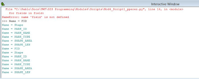
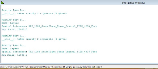
This week’s assignment covered debugging and error handling in PythonWin using the debugger and the try-except statements.  The first and second script contained errors that were identified by running the debugger on a step by step (line by line) to correct the errors based on the error message information and codes provided by PythonWin.  The third script contained errors but the errors were not corrected.  Instead the try-except statements were used to capture the error and to print the error messages thus allowing the code to run with the errors.

Below is are screenshots of the interactive window results for the three scripts.

GIS 4102: GIS Programming Module 3

Module 3: Python Fundamentals Part 2

This week’s assignment covered importing modules, correcting script errors, creating while loops and conditional statements, adding script comments, and iterating variables within a loop.  The script performs a little dice rolling game based on the player’s name length, then creates a list with 20 random numbers in it.  The script also creates a conditional statement with a nested while loop that removes all instances of a specified number in the list.

The script imports the random module and uses the following functions and methods:

·         Len function.

·         Random integer method.

·         List append method.

·         List count method.

·         List remove method.

Below is a screen shot of the results of the script.